Scenario computation
FPP allows, for a given script, to parallelize on documents (as in the previous section) but also on scenarios and calculation dates. In this section, you will parallelize on scenarios by modifying the pricing data file.
To generate scenarios, we added two new fields to the input file: shiftsIncluded and shifts.
To find out more about executing scripts in parallel, follow the Parallelization tutorial from the Financial Model Builder Documentation.
Scenario Workflow Files
Java Class
Open the Tutorial_portfolio.java class file, and remove the multi-line comments around shift.
You can download the uncommented Java file here.
Box file
Open the tutorial_Portfolio.box file, and remove the multi-line comments around Scenario generation and Prepare Output.
Scenario generation: Creates new scenarios according to the information of the
shiftssection. It will also add information about the shifts and the percentage applied.Prepare Output: Computes the
PVs per secondindicator, which is the number of present value operations done per second.
You can download the uncommented box file here.
Input File
Add to the tutorial_PortfolioInput.json file the two new fields
shiftsIncluded and shifts:
{
  ...
  "shiftsIncluded" : true,
  "shifts": [
    {
      "type": "YIELD_CURVE",
      "param1": "projection_Libor_3M",
      "param2": "discountFactor",
      "min": -10,
      "max": 10,
      "steps": 3
    }
  ]
}
You can download the uncommented input file here.
The
shiftsIncludedfield is a Boolean flag indicating if scenario generation has to be done.- The
shiftsfield contains the following information:- type: Type of the considered Scenario Identifier.
- param1 and param2: Parameters of the considered Scenario Identifier.
- min and max: The lower and upper percentage change in the Scenario Values associated with the considered Scenario Identifier.
- steps: Number of steps between min and max.
The total number of scenarios is given by:
\[\begin{equation} {{\#scenarios} = initial\, scenario + {steps} + {1}} \end{equation}\]
In the below example with 3 steps, we will have 5 scenarios computed:
\[\begin{equation} {S_i\,, i\,\epsilon\, [0,4]} \end{equation}\]
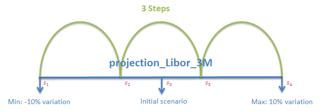
Fig. 106: Scenario generation.
In our case, the scenario identifier is the yield curve projection_Libor_3M expressed as discount factor.
To generate new scenarios on this yield curve, the original discount factor is converted to a zero coupon rate, modified according to the shift values (percentage change) and then converted back to discount factor.
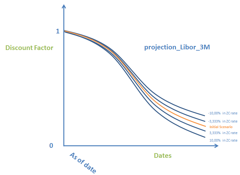
Fig. 107: Data modification.
The complete scenario generation process is described below:
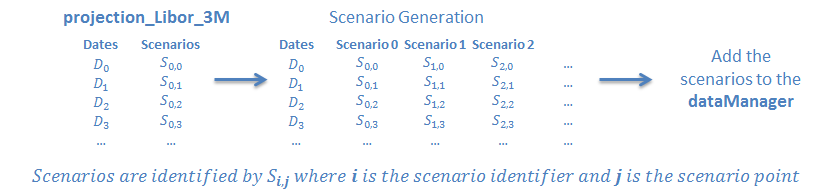
Fig. 108: Yield curve scenario generation.
Our portfolio pricing data file contains one single scenario.
Execute the Workflow in the Financial Model Builder Editor
Execute the
tutorial_Portfolioworkflow after the previous modifications.The result shows the information about the scenarios, the present value for each of them and the
PVs per second.
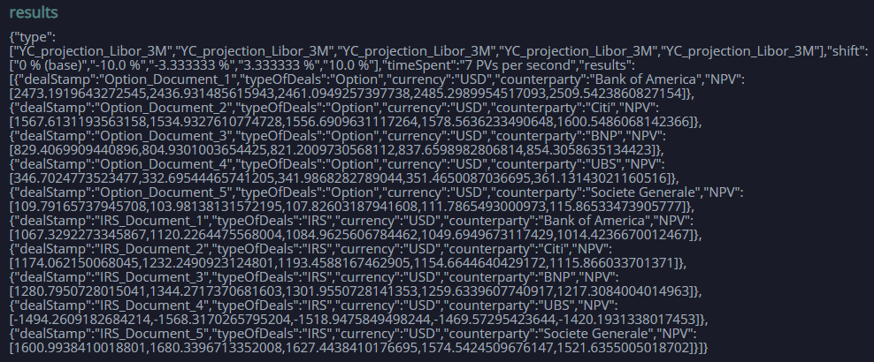
Fig. 109: Workflow results.
Execute the Workflow in REST mode
Execute the workflow in Microsoft Excel
In Financial Model Builder deploy your libraries.
Open the tutorial_PortfolioValuation_App.xlsm and set up your connection.
Ungroup the rows after the
inputIncludedcell and unhide the Device tab:
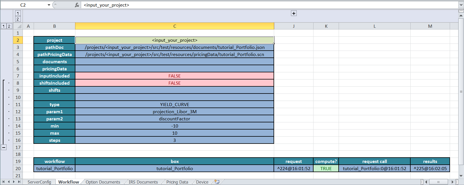
Fig. 110: Scenarios section in Microsoft Excel.
- Set shiftsIncluded to
true, and then click Recompute All. The flag and the information about the shifts are included in the request to the Financial Model Builder.
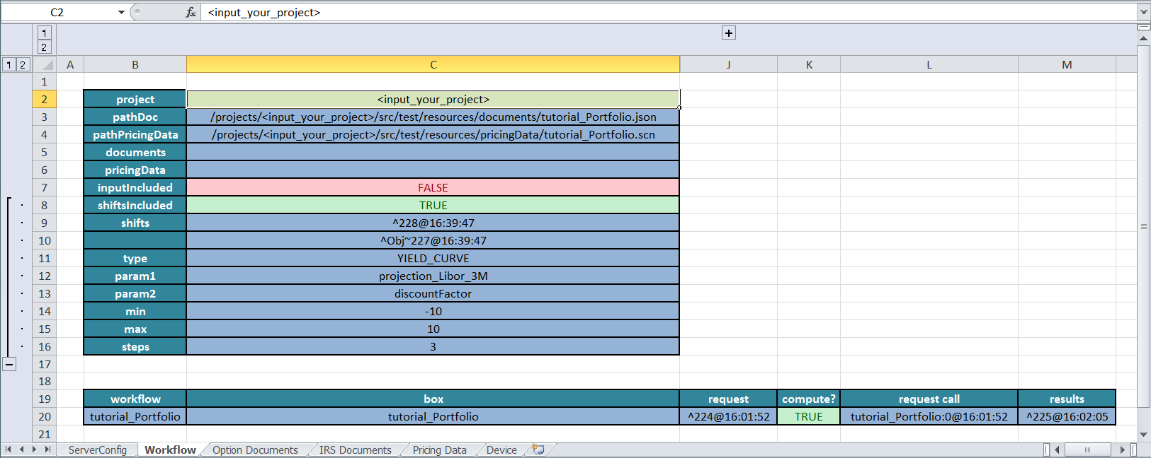
Fig. 111: Scenarios using Microsoft Excel.
- To see the results, select the results reference and either click
Open JSON in Editorfrom the Valuation ribbon or right-click to use the contextual menu.
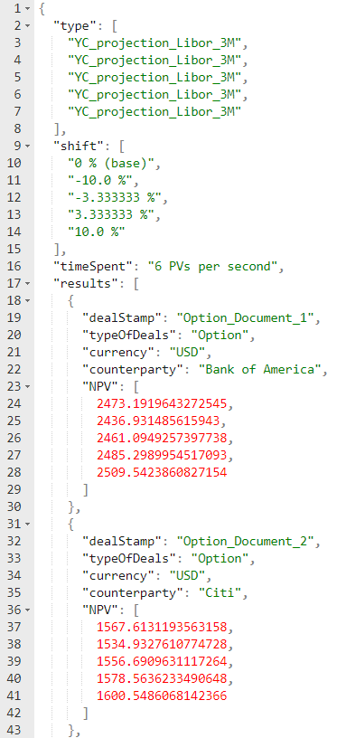
Fig. 112: Workflow results in editor.
Device: It allows you to choose the device of the execution (Groovy, Java, SIMD CPU or even GPU for advanced users). For SIMD CPU or GPU devices, the parallelization will be done automatically, improving the performance.
Visualize the Scenarios Data
Go to the FusionCreator App Builder, create a new board and name it Scenarios.
Create the Scenarios Cube
- Switch to Data management page.
- Click CSV DATA IMPORT.
- Click Open CSV editor.
- Copy the following lines and paste them in the CSV Editor
dealStamp:PK;type:PK;shiftId:PK;shift;NPV;NPVchange;counterparty;currency;typeOfDeals
string;string;string;fixed_decimal[4];double;double;string;string;string- Enter the Cube Name:
PortfolioValuationScenarios, and then click Import. You have just created an empty cube that is waiting to be populated with data. - Click Generate the report. The Report Name field is automatically filled with the name of the cube. You can change it, but take a note of it as you will use it to select the data source in all the subsequent data visualization.
Create the Scenarios Flow
- Switch the UI to Flow editor mode.
- Go to the Portfolio Valuation flow.
- From the Flow Menu select Import > Clipboard.
- Copy the following code, and paste it into the text area of the Import nodes window. Select Import to current flow.
[
  {
    "id": "555b904f.a0cf5",
    "type": "mb-http-in",
    "z": "587ece37.e4e0b",
    "name": "Scenarios",
    "x": 100,
    "y": 100,
    "wires": [
      [
        "9db9923a.93e5a"
      ]
    ],
    "method": "post",
    "url": "/24f1a8f7-8536-255a-dcc9-8194a5412b2d/"
  },
  {
    "id": "9db9923a.93e5a",
    "type": "mb-notifier",
    "z": "587ece37.e4e0b",
    "name": "Clear_Stats",
    "x": 110,
    "y": 220,
    "wires": []
  },
  {
    "id": "3dc1aa05.9e3926",
    "type": "function",
    "z": "587ece37.e4e0b",
    "name": "PVs per second",
    "func": "if (!msg.req.url.includes('Calculate')){\nmsg.payload ='<!DOCTYPE html><html><body><p></p><h2><center>$heading</center></h2><p></p></body></html>'\nmsg.payload = msg.payload.replace('$heading', msg.time) \nreturn msg;\n }",
    "outputs": 1,
    "noerr": 0,
    "x": 820,
    "y": 100,
    "wires": [
      [
        "291a06df.397a2a"
      ]
    ]
  },
  {
    "id": "291a06df.397a2a",
    "type": "mb-notifier",
    "z": "587ece37.e4e0b",
    "name": "Stats",
    "x": 1010,
    "y": 100,
    "wires": []
  },
  {
    "id": "cb5b493f.0154c8",
    "type": "mb-http-out",
    "z": "587ece37.e4e0b",
    "name": "Scenarios_out",
    "x": 820,
    "y": 300,
    "wires": []
  },
  {
    "id": "8c5d7be1.96a9c8",
    "type": "mb-http-in",
    "z": "587ece37.e4e0b",
    "name": "ResetScenarios",
    "method": "post",
    "url": "/c52116fc-3b3e-10c6-626e-39b32a8debca/ResetScenarios",
    "x": 120,
    "y": 480,
    "wires": [
      [
        "feb08388.1d8b8"
      ]
    ]
  },
  {
    "id": "feb08388.1d8b8",
    "type": "cube-delete",
    "z": "587ece37.e4e0b",
    "default": true,
    "deleteRowsInCube_id": "PortfolioValuationScenarios",
    "deleteRowsInCube_idType": "str",
    "deleteRowsInCube_filter": "",
    "deleteRowsInCube_filterType": "nof",
    "name": "Reset Cube",
    "x": 330,
    "y": 480,
    "wires": [
      [
        "d3db1546.750de8"
      ]
    ]
  },
  {
    "id": "d3db1546.750de8",
    "type": "mb-http-out",
    "z": "587ece37.e4e0b",
    "name": "ResetScenarios_out",
    "x": 560,
    "y": 480,
    "wires": []
  }
]- Connect the new nodes to the main flow as below:
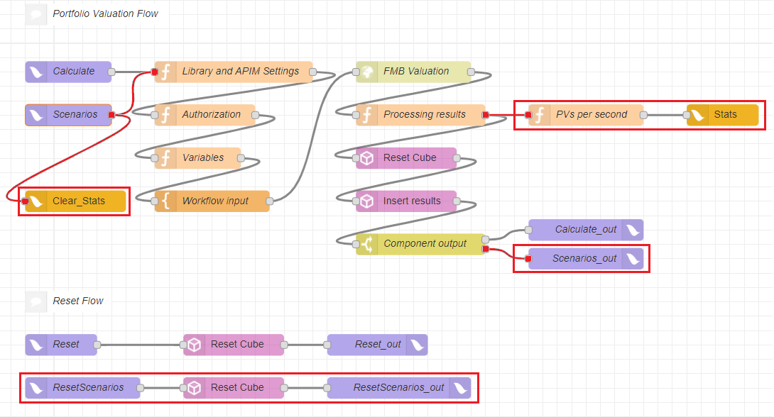
Fig. 113: The updated flow in Flow editor.
- Click Deploy to make your flow available in the Components list of the UI.
Connect the flow with the UI
To connect the flow with the UI
- Switch the UI to Design mode.
- Add a form to the board and configure it as follows:
- Title:
Scenario selection - Go to Schema and paste the following code:
- Title:
{
  "title": "Scenario selection",
  "type": "object",
  "properties": {
    "Yield Curve": {
      "type": "string",
      "enum": [
        "projection_Libor_3M",
        "discount_Libor_3M"
      ]
    },
    "Min": {
      "default": -10,
      "type": "number",
      "minimum": -100,
      "maximum": 100,
      "description": "Lower percentage"
    },
    "Max": {
      "default": 10,
      "type": "number",
      "minimum": -100,
      "maximum": 100,
      "description": "Higher percentage"
    },
    "steps": {
      "default": 3,
      "type": "number",
      "minimum": 1
    },
    "Device": {
      "type": "string",
      "default": "SIMD CPU",
      "enum": [
        "SIMD CPU",
        "JAVA",
        "GROOVY"
      ]
    }
  }
}- Go to Actions and create two actions,
Calculate ScenariosandReset Scenarioswith the same Display and Action name.
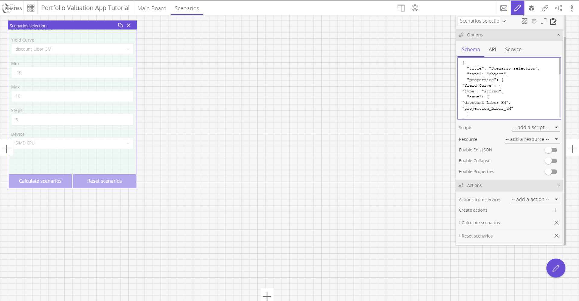
Fig. 114: Form to select the scenarios.
- Switch the UI to Link editor mode.
- On the Components bar click Reuse.
- Select the Scenario selection form that you just created in the Layout editor. A box listing the actions and events bound is displayed on the board.
- Connect the
Calculate Scenariosevent of the Scenario selection form to the Scenarios action of the Portfolio Valuation flow. The effect of this link is that when you click the button, you trigger the flow in Flow editor which, in turn, calls Financial Model Builder to execute thetutorial_Portfolioworkflow. - Repeat the step 6 for the
Reset Scenariosaction.
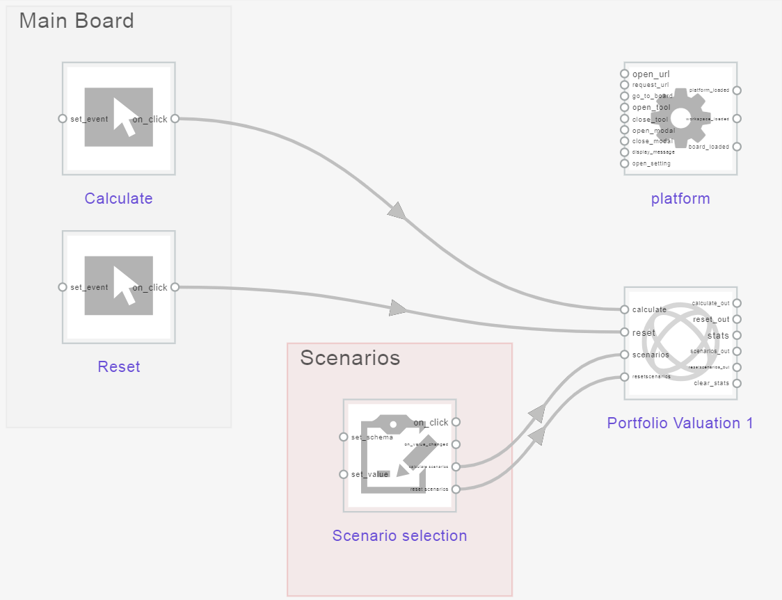
Fig. 115: Link editor.
Display Results
To display the results in a table
- Switch the UI to Design mode.
- Add a new table to the board and configure it as follows:
- Title:
Portfolio Deals - Data source: select the
PortfolioValuationScenariosreport - Columns: Click on
Select All
- Title:
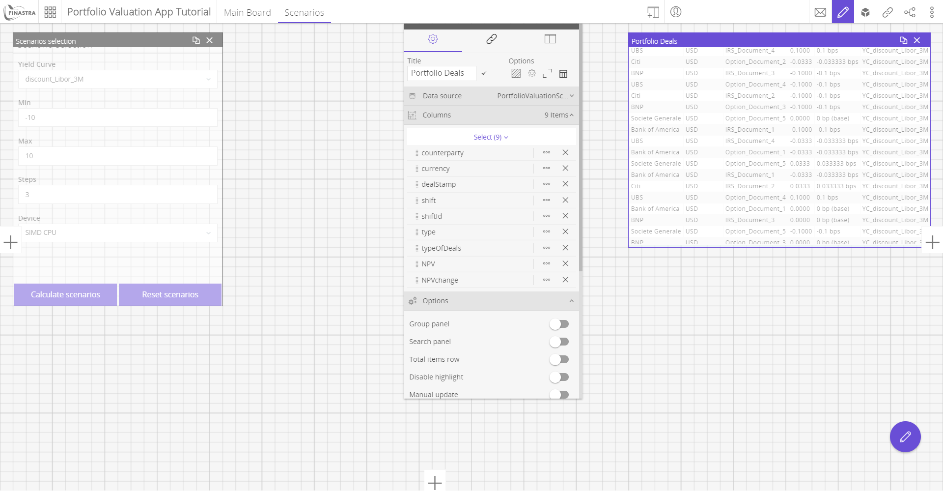
Fig. 116: Table showing all the results.
To create a Chart showing the change in NPV per deal simultaneously
- Switch the UI to Design mode.
- Add a new Pie Chart to the board and configure it as follows:
- Title:
NPV change - Data source: select the
PortfolioValuationScenariosreport - Horizontal axis: select
shift - Vertical axis: select
NPVchange - Series: select
dealStamp - Chart type: select
Spline
- Title:
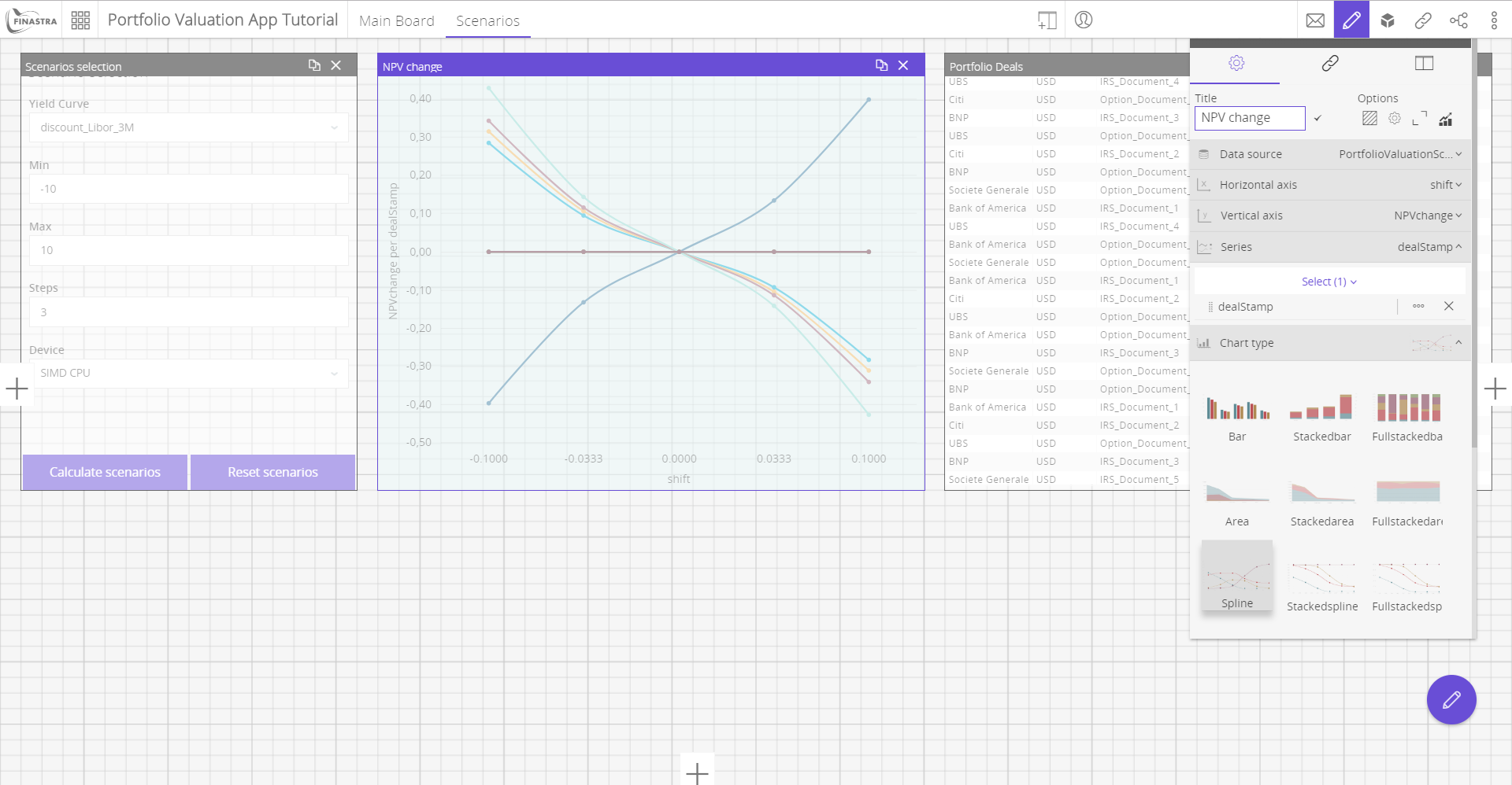
Fig. 117: NPV change.
To create a Smart View showing the change in NPV per deal
- Switch the UI to Design mode.
- Add a new Smart View to the board and configure it as follows:
- Title:
NPV changes per deal - Dimensions: select
dealStampandshift - Measures: select
NPVchange - Chart type: select
Bar
- Title:
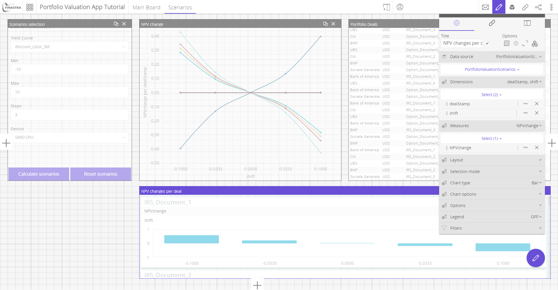
Fig. 118: NPV changes per deal.
To create a componentEditor component showing the execution time
- Switch the UI to Design mode.
- Add a new componentEditor component to the board and configure it as follows:
- Pens selection: Blank
- Title:
Stats - JS: In the JS editor, copy and paste the following code:
mbCoreIframe.utils.addListener('STATS', function(data){
document.body.innerHTML = data.value;
});
mbCoreIframe.utils.addListener('CLEARSTATS', function(data){
document.body.innerHTML = '';
});
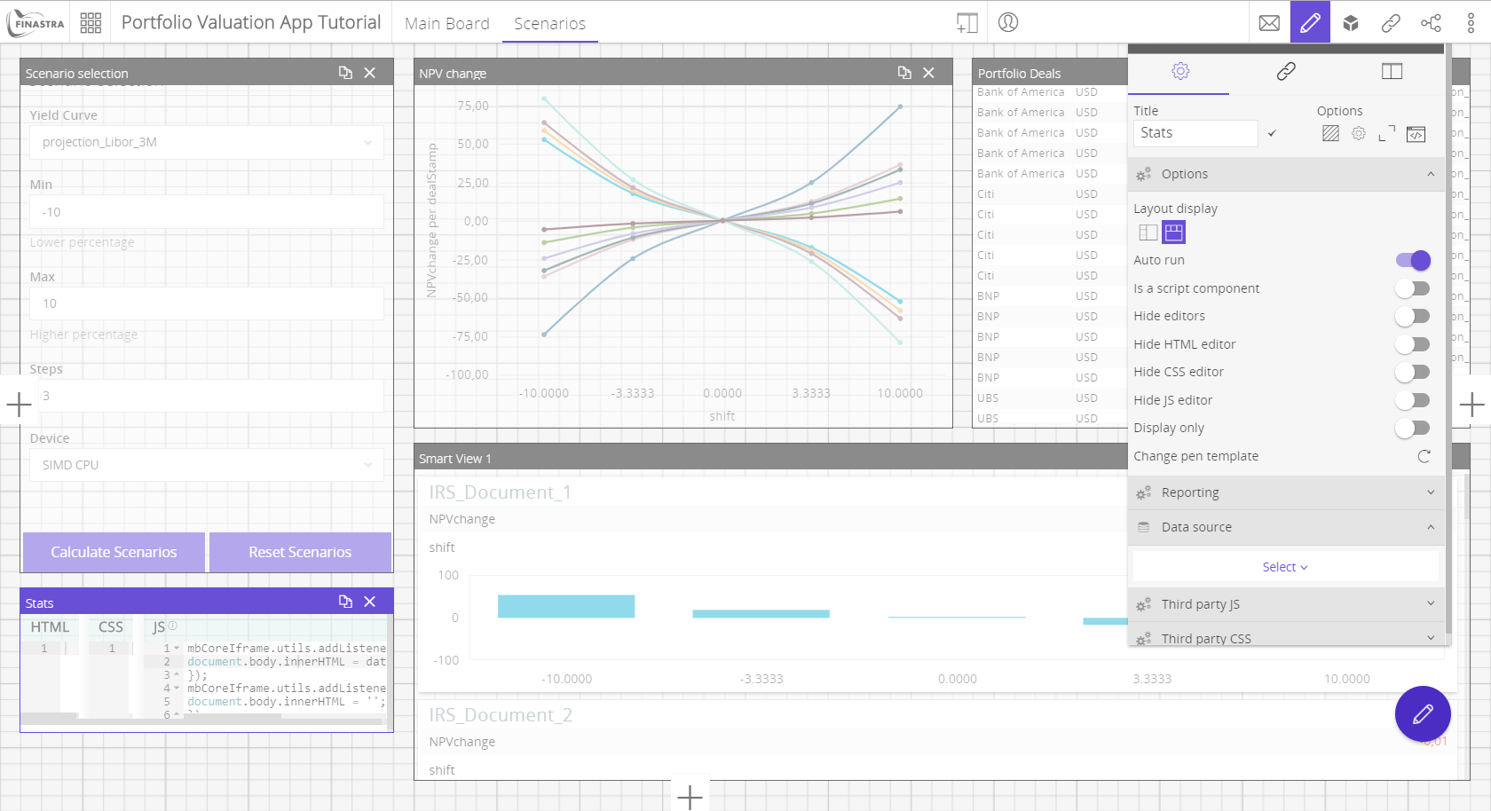
Fig. 119: PVs per second.
Finally, turn on the Display only option.
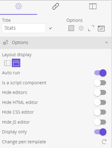
Fig. 120: Display only option.
- Connect now the
Statscomponent to the flow as below:
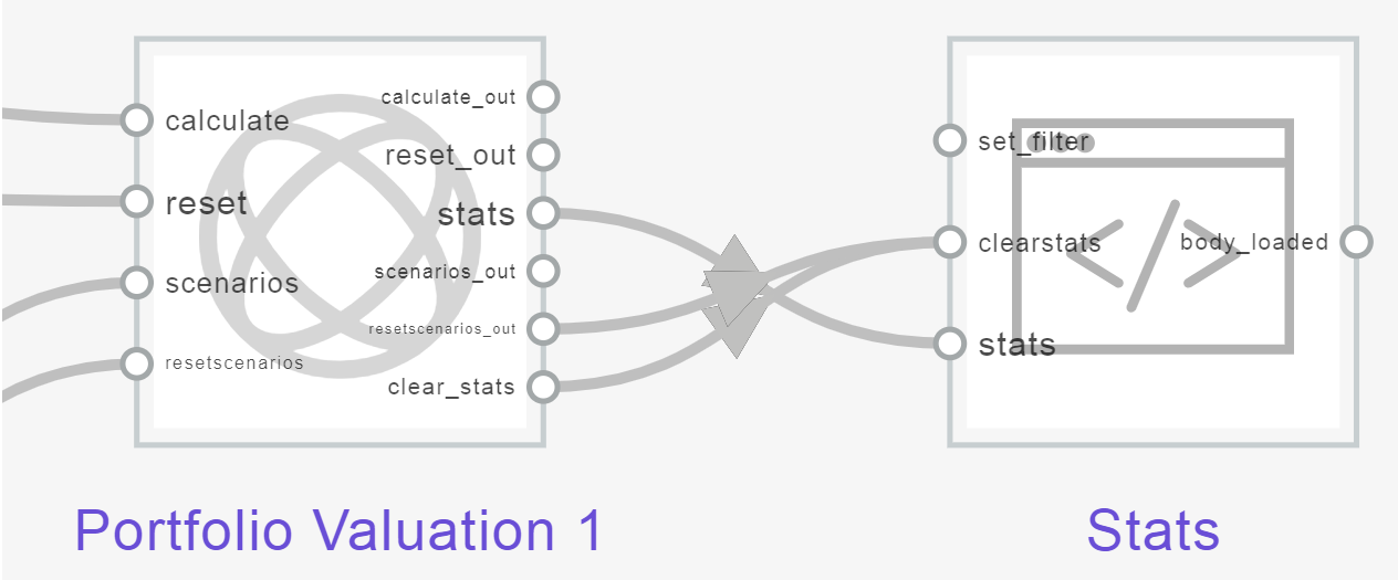
Fig. 121: PVs per second link.
Run the Portfolio Valuation App
To run the Portfolio Valuation App
- Deploy your libraries in the Financial Model Builder.
- Click on the Calculate Scenarios button, this will:
- Restore the results in the
PortfolioValuationScenarioscube. - Display the results in the four components.
- Restore the results in the
- Click on the Reset Scenarios button to delete the content of the
PortfolioValuationScenarioscube.
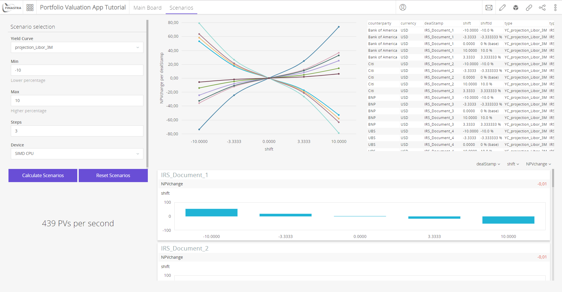
Fig. 122: Complete view of the Portfolio Valuation App with scenarios.